Re: Slur with left and/or right arrow head

[Aaron Hill]

On 2019-04-17 3:31 pm, Thomas Morley wrote:
> Well, I'd like to understand beziers better, continuing my afford here
> also means I shouldn't ignore such things ;)

Beziers are one way to generalize simple linear interpolation to higher 
orders, and they have a rather curious recursive relationship which my 
code exploits.

In linear interpolation, we only have two control points.  We want to 
move from point A to point B along the lowest order path, which must be 
a straight line.  This can be written as a weighted average of the two 
points using a interpolation factor:

  f(t) = A (1 - t) + B t

The parameter, t, in the above form would go from zero to one to 
interpolate.  (And if you go outside that domain, you are then 
extrapolating.)  When t is zero, the value B is eliminated whereas A is 
left intact.  When t is one, the opposite occurs.  Finally, when t is 
one half, t and (1 - t) are the same leading to an equation: (A + B) / 
2, which is exactly the midpoint of two values.

It should be noted that when I say "point", I am not prescribing any 
particular dimension.  We can use linear interpolation against 
one-dimensional scalars just as easily as seventeen-dimensional vectors. 
 When you have more than one component, all you need to do is 
interpolate each component independently:

  x(t) = A.x (1 - t) + B.x t
  y(t) = A.y (1 - t) + B.y t
  z(t) = A.z (1 - t) + B.z t
  etc.

For higher order Beziers, we are doing nothing more than a weighted 
average of all of the control points.  Here are the second and 
third-order forms:

  f(t) = A * (1 - t)^2 + 2 B (1 - t) t + C t^2
  f(t) = A * (1 - t)^3 + 3 B (1 - t)^2 t + 3 C (1 - t) t^2 + D t^3

There are two interesting patterns here, which makes it very easy to 
remember these equations.  First, note that the exponents of (1 - t) and 
t are decreasing and increasing, respectively, between the terms.  
Second, the additional scalar coefficients come from rows of Pascal's 
triangle:

      1
     1 1
    1 2 1    <-
   1 3 3 1   <-
  1 4 6 4 1

Looking at the equations above, the first point is affected entirely by 
(1 - t); the last, entirely by t.  All points between involve both (1 - 
t) and t.  As such, when t is zero, all terms except the first are 
cancelled out; and similarly, all terms but the last are cancelled out 
when t is one.  For values between zero and one, we get some average of 
the points.  The implication here is that, though we strictly begin and 
end at the first and last points, the path we take might not pass 
through any of the middle control points.

There is no limit to how many control points you would like to 
accommodate.  However, it can be a little cumbersome to write out the 
equation for higher orders.  This is where a little bit of recursion can 
help.

Bezier curves need only use linear interpolation to compute the result.  
Let's consider the second-order case first.  We have three control 
points: A, B, and C.  Using the parameter, t, linearly interpolate 
points A and B, labelling that AB.  Next, do the same for points B and 
C, labelling it BC.  We now have reduced three points to only two.  
Finally, linearly interpolate AB and BC, and the result is exactly what 
we want:

  AB = A (1 - t) + B t
  BC = B (1 - t) + C t

  ABC = AB (1 - t) + BC t
      = [ A (1 - t) + B t ] (1 - t) + [ B (1 - t) + C t ] t
      = A (1 - t)^2 + B t (1 - t) + B (1 - t) t + C t^2
      = A (1 - t)^2 + 2 B (1 - t) t + C t^2

The same approach works for higher orders.  My recursive function 
achieves this by taking a list of control points and defining two new 
lists: one that omits the last element and another that omits the first 
element.  These new lists are Bezier curves of a lower order.  The 
process continues until the list is simply two points, which is nothing 
more than linear interpolation.

Regarding the parameter, t: if you imagine that you are walking a path 
from the first point to the last point, then thinking of t as "time" 
should make sense.  The trick, I suppose, is that this is not absolute 
time but relative time.  That is, think of t as a percentage of the 
entire journey.  At zero (0%), we have just begun to walk and are 
standing at the first point; and at one (100%) we have just finished 
walking and are located at the final point.  Again, technically we can 
exceed this range.  For negative values, we are talking about what 
happened *before* we began walking at the first point.  And for values 
above one, we are continuing to walk beyond the final point.  The Bezier 
curve is infinite, though we often only consider the segment defined by 
the interval [0, 1].

Additionally, it is important to consider velocity along the curve.  
Based on the positioning of the control points, we may be walking at 
times and running at others.  You see this with the variable spacing of 
dots when you sampled a curve at regular intervals of the parameter t.  
A value of one half for t does not mean you are halfway between the 
initial and final points in terms of Cartesian distance.  This is why I 
had to go through the trouble of computing arc lengths, since I needed 
to know the slope of the curve at a specific distance from the end 
points.

My approximation for arc length and position will fail for exotic Bezier 
curves, since I am using a fixed subdivision count; but typically ties 
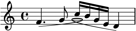
and slurs are more well-behaved in this regard.  Now when a composer 
decides to invent notation where a slur has a cusp or loop in it, then 
we will need to worry:

%%%%
\version "2.19.82"

\fixed c' {
  f4.
    -\tweak thickness #2
    -\offset control-points
      #'(((0 . 0) (24 . 4) (-24 . 6) (0 . 0)))
    ( g8 c'16 b g e d4)
}
%%%%

> Am Mi., 17. Apr. 2019 um 22:53 Uhr schrieb David Kastrup <address@hidden>:
> > [ . . . ] It's just trying to give an artifical
> > construct in the form of an independent arbitrary parameter that has
> > been arbitrarily normalized from 0 to 1 (and indeed, in LilyPond a
> > normalization from -1 to 1, namely #LEFT to #RIGHT might be better
> > justifiable but diverging from most formulas in literature) some more
> > tangible image/meaning.

It is pretty simple to adapt the equations above to accommodate an 
interval of [-1, 1].  Our new parameter, s, can be converted to t as 
such:

  t = (s + 1) / 2

So linear interpolation of A and B, in terms of s, becomes:

  f(s) = [ A (1 - s) + B (1 + s) ] / 2

When s = -1, (1 - s) becomes 2 and (1 + s) becomes 0.  Likewise, when s 
= 1, (1 - s) is 0 and (1 + s) is 2.  Finally, when s = 0, both (1 - s) 
and (1 + s) are 1.  We do need to apply a scalar 1/2 to the whole thing, 
but otherwise it works the same.


-- Aaron Hill

funny-slur.cropped.png
Description: PNG image